Mapping zipcodes in R

I started fiddling around with R again, and ended up playing with a zipcode database.

So, first I downloaded the zipcode database at Mapping Hacks, and unpacked the zipfile in my working directory.

Then, I loaded the data into R

> zips <- read.table("zipcode.csv",sep=",",quote="\"",header=TRUE)
> names(zips)
[1] "zip"       "city"      "state"     "latitude"  "longitude"
[6] "timezone"  "dst"

So, now I have an R frame containing a lot of US cities, their geographical coordinates, and their zip codes. So we can start playing with the plot command! After rooting around a bit, I ended up settling on the smallest footprint plot dot I could make R produce, by setting the option pch=20 in the plot options. Hence, I ended up with a command basically like this:

> plot(zips$longitude,zips$latitude,type="p",col=((zips$zip/10000)%%10)+1,pch=20,axes=FALSE,xlab="",ylab="",cex=0.1)

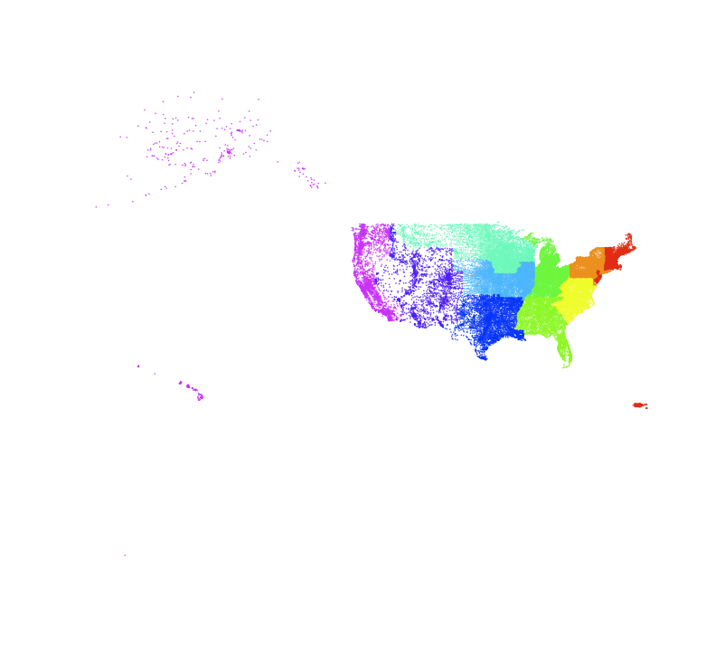
where the +1 after the modulus is to make even 0-values plot, and the cex parameter sets the point size to something small and pretty.

We can continue this, tweaking the divisor to extract all the other digits of the zip code, and we end up getting:

> plot(zips$longitude,zips$latitude,type="p",col=((zips$zip/1000)%%10)+1,pch=20,axes=FALSE,xlab="",ylab="",cex=0.1)

and the result

> plot(zips$longitude,zips$latitude,type="p",col=((zips$zip/100)%%10)+1,pch=20,axes=FALSE,xlab="",ylab="",cex=0.1)

and the result

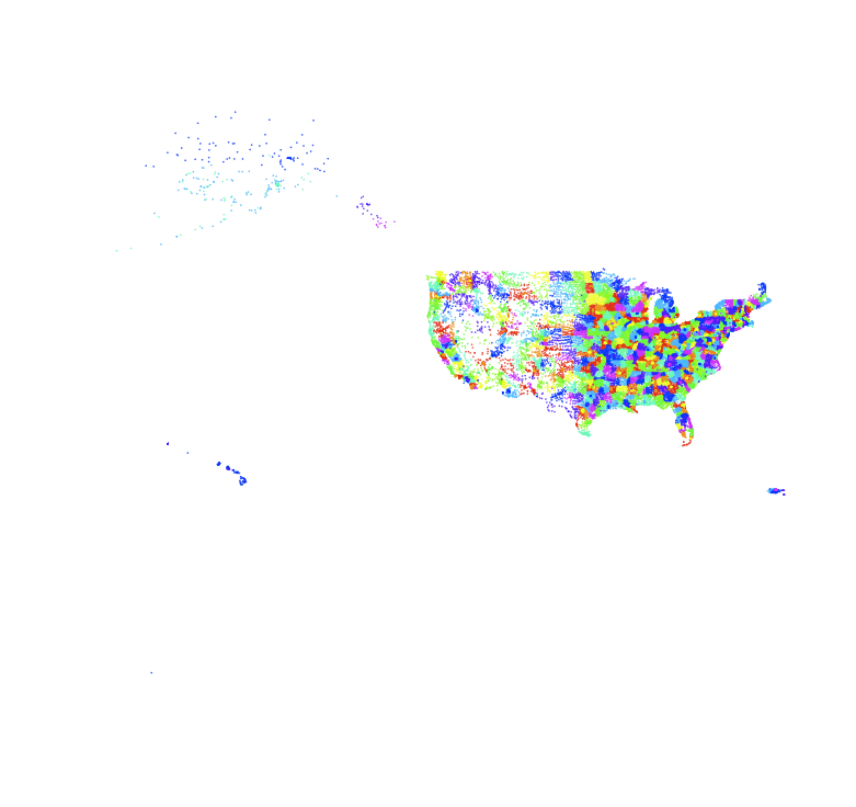
> plot(zips$longitude,zips$latitude,type="p",col=((zips$zip/10)%%10)+1,pch=20,axes=FALSE,xlab="",ylab="",cex=0.1)

and the result

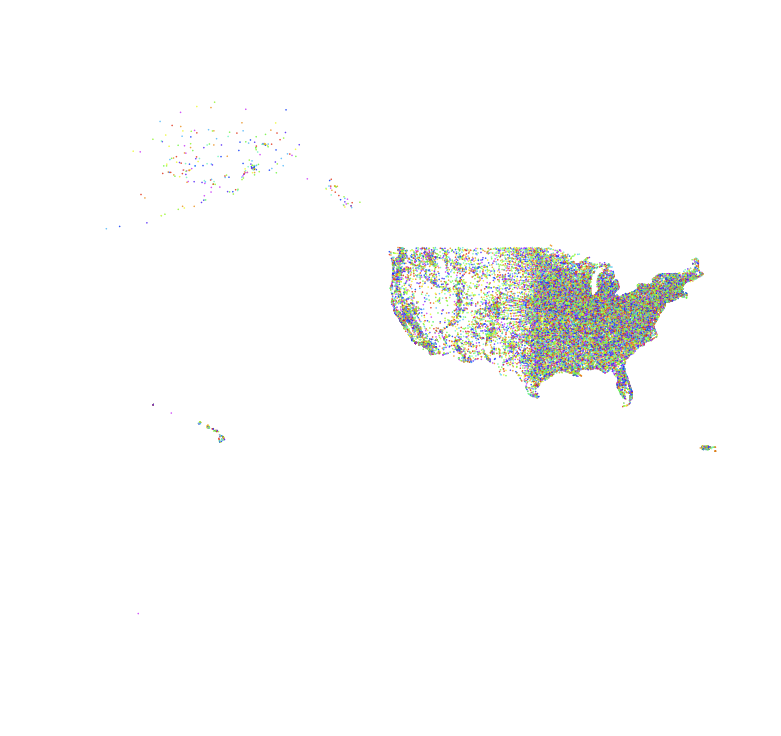
and finally

> plot(zips$longitude,zips$latitude,type="p",col=((zips$zip/1)%%10)+1,pch=20,axes=FALSE,xlab="",ylab="",cex=0.1)

and the result

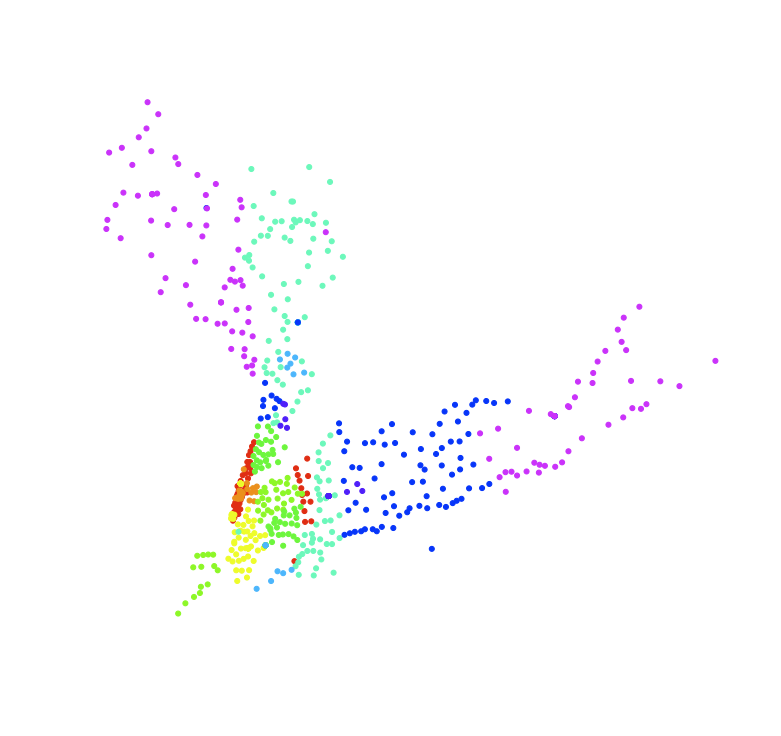
And then, of course, we can zoom in on data too. So we can do things like extracting Californian zip codes

> cazips <- zips[zips$state == "CA",]
> plot(cazips$longitude,cazips$latitude,type="p",col=((cazips$zip/1000)%%10)+1,pch=20,axes=FALSE,xlab="",ylab="",cex=0.5)

to get

Second digit of the Californian USPS zip code

or, we could extract New York zip codes:

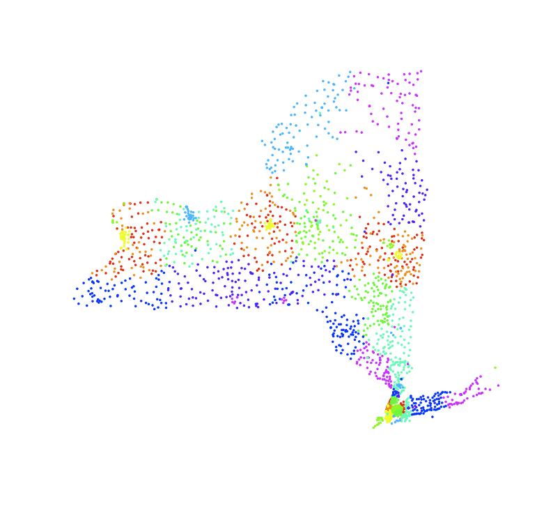
> nyzips <- zips[zips$state == "NY",]
> plot(nyzips$longitude,nyzips$latitude,type="p",col=((nyzips$zip/100)%%10)+1,pch=20,axes=FALSE,xlab="",ylab="",cex=0.5)

Third digit of the New York USPS zip code

or even extract, say, the zip codes starting with 10 or 11, covering New York City and surroundings and take a closer look

> ny10zips <- nyzips[nyzips$zip<12000,]
> ny10zips <- ny10zips[ny10zips$zip>9999,]
> plot(ny10zips$longitude,ny10zips$latitude,type="p",col=((ny10zips$zip/100)%%10)+1,pch=20,axes=FALSE,xlab="",ylab="",cex=1.0)

social