1st: What do we mean by political data?

We currently look at 3 types of data:

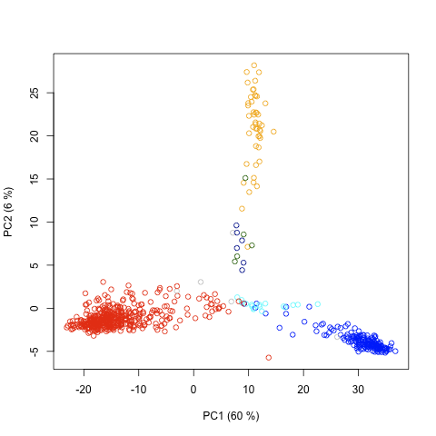
1. Vote matrices from parliament:

   each column is a member of parliament each row is a rollcall we codify votes numerically: +1/-1 for Yea/Nay

   And then we can do data analysis either on the set of members of parliament in the space of rollcalls, or on the set of rollcalls in the space of members of parliament.

2. Co-sponsorship graphs

   Nodes are members of parliament.

   A directed edge goes from each co-sponsor to the main sponsor of a particular bill, for all bills.

   For Swedish politics, parties end up being strongly connected internally, with coalition mediators appearing in the data.

3. Shared N-gram graphs

   Some turns of phrase, some talking points, get introduced and then re-used by other members of parliament.

   We believe that an analysis of N-grams of parliamentary speeches may well give a data analyst tools to capture memetic drift and spread within partliament.

The project is still at an early stage, and the great challenge for us right now is to find value to add — in political science, the grand entrance of classical data analysis was a few decades ago, and much of what can be said about politics with classical data analysis tools has already been said.

2nd: What has already been done?

Political science discovered data analysis in the 90s, and a flurry of political science data analysis papers followed.

Thus, while illustrative, doing things like a PCA on political vote data is not quite novel.

Doing these PCAs, though, shows us, for instance, that the US house & senate are essentially linear,

and that the votes point cloud sits on most of the boundary of a unit square (above right): at least one party backs every bill that comes to a vote, and the main difference between bills is in how many of the other party join in too.

Already in this kind of analysis, we notice a difference over time — the party line is a much stronger factor in 2009 than it was in 1990:

We can perform similar analyses for the UK:

Here we may notice that the regional parties are pretty much included with the ideologically closest major party. This is a phenomenon we're going to revisit later on.

With Swedish vote data, we've been able to both locate the blocks as essentially grouped under the first two coordinates of a PCA; with lower coordinates seemingly issues-oriented — it's worth noticing component 5 which separates out C and MP from the other parties, and thus seems to be the axis of environmentalism in Swedish politics.

image courtesy of Anders Sandberg

3rd: How do we bring in topology?

There are several techniques developed at Stanford for topological data analysis. While my own research has been centered around persistent homology, the one I want to present here is different.

Mapper was developed by Gurjeet Singh, Facundo Memoli and Gunnar Carlsson. It builds on combining nerves with parameter spaces.

Now, if X is a topological space with a coordinate function [tex]X\xlongrightarrow{f}Z[/tex] and Z is (paracompact and) covered by some family of [tex]U_i[/tex], then the collection of preimages covers X.

So, by subdividing each preimage of a set in the covering of Z into its connected components, we get a covering of X subdividing the cover induced from Z.

Thus, if f is sufficiently wellbehaved and the covering is fine enough, the nerve of these subdivided preimages is homotopy equivalent to X, and we have found a triangulation (up to homotopy) of X.

This technique has been used already to recover the difference between diabetes type I and II as lobes in the data, apparent in blue here:

We hope to be able to use these techniques to better understand the way parliaments are structured internally.